Implicit Solvation Models: COSMO (CPCM), PCM (DPCM), IEFPCM¶

Figure 1: Temperature-Pressure phase diagram ¹

Introduction to thermodynamics¶

The chemical potential is an important theoretical quantity in the field of thermodynamics and describes the change in energy of a chemical system of multiple components where the composition of a system is under change.

The composition of atoms or molecules in the system can change due to a reaction or due to a flux between the system/phase boundaries. Common examples of such chemical phenomena can be observed in our environment or in industrial processes (Figure 1).

The chemical potential can be related to thermodynamic state functions, namely internal energy \(U(S,V)\), enthalpy \(H(S,p)\), Helmholtz energy \(F(T,V)\), Gibbs enery \(G(T,p)\):

\[dU = TdS − pdV + \sum_i \mu_i dni\]

\[dH = TdS − VdT + \sum_i \mu_i dni\]

\[dF = -pdV - TdS + \sum_i \mu_i dn_i\]

\[dG = Vdp - SdT + \sum_i \mu_i dn_i\]

and one can derive that:

\[\mu_i = (\frac{\delta G}{\delta n_i})_{p,T,n_j}\]

Phase equilibria calculations such as vapour liquid equilibria (VLE), liquid liquid equilibria (LLE), solid liquid equilibria (SLE) are states where the chemical potentials of all the phases are equal:

\[\mu_i^j = \mu_i^l\]

With this quick recap of some basic thermodynamic equations we will move on to discuss the theory of implicit solvation models and circle back to the connection between solvation models and thermodynamic properties in the end of the solvation models section.

Solvation models¶

When considering the environment of an atom or molecule in solution, then the electronic effect of the atoms/molecules surrounding an atom/molecule of interest needs to be taken into account.

Implicit solvation models describe this interaction between a solute and a solvent with considering a polarizable continuum (also called dielectric medium). This electronic spatial profile of molecules allows to map a profile of positive and negative charge distributions on a specific surface around the solute molecule. This profile is called the apparent surface charge (ASC) density \(\sigma(\vec{s})\) and defines a border between the solute and the continuum of the solvent. The polarity of the solvent will have an influence on the ASC density and the polarity is defined with the dielectric constant \(\epsilon(\vec{r})\).

The electrostatic solvation energy of a molecule in solutions is defined as:

\[G^{el}_{solvation} = \frac{1}{2} \int_s \sigma(\vec{r}) \phi(\vec{r})\]

and is the change in energy when transferring the molecule under consideration from the gas phase into the solution/solvent(s) phase. The integration is performed over the solute surface points \(s\).

To retrieve the before mentioned apparent surface charge (ASC) density \(\sigma(\vec{r})\) of the solute molecule, the Poisson equation has to be solved ²:

\[ \nabla [\epsilon(\vec{r}) \nabla \phi(\vec{r})] = - 4 \pi \rho(\vec{r})\]

Where the equation simplifies with \(\epsilon(r) = 1\) within the solute molecule cavity to:

\[ \nabla^2 \phi(\vec{r}) = - 4 \pi \rho(\vec{r})\]

and with \(\epsilon(r) = \epsilon\) (set to a constant value, e.g. to 80 for water) outside of the solute cavity to:

\[ \epsilon \nabla^2 \phi(\vec{r}) = 0 \]

There exist different ways how the Poisson equation can be solved where the electrostatic surface around the molecule is dissected into smaller pieces (tesserae). The Poisson equation is then being solved in combination with a tesserae dissection routine.

In this article we present the DPCM, CPCM/COSMO and IPCM/IEFPCM models which differ based on the implemented boundary conditions. Important to highlight is that the DPCM model relies on the net electric field, \(E_n\), and the COSMO and IEFPCM models depend only on the net potential (\(\phi(s)\)) at the cavity surface of a given solute molecule ³. IEFPCM reduces to the COSMO model when \(\epsilon\) approaches infinity ⁴.

To solve the Poisson equation numerically and to provide a general mathematical formulation, one can recast the equation in matrix form:

\[\vec{q} = \mathbf{K} \vec{f} \]

with \(\vec{q}\) storing the unknown cavity surface charges, \(\mathbf{K}\) (the solvent response matrix) being a square matrix storing the information about the geometry (tesserae location, area) and dielectric information of the medium.

\(\mathbf{K}\) is defined by the matrices/operators \(\mathbf{A}\), \(\mathbf{D}\) and \(\mathbf{S}\) presented later. \(\vec{f}\) holds the normal component of the electrostatic quantity at the tesserae. Tomasi et al. ³ provide a nice overview (Table 1 in the publication) how this equation in matrix form can be utilized to calculate the ASC density with various methods (e.g. PCM/DPCM, CPCM/COSMO, IEFPCM).

The DPCM ASC density \(\sigma(\vec{s})\) defintion with the exact dielectric boundary condition (EDBC) at the interface (surface) of the cavity, with \(\vec{s}\) being a point on the cavity surface, is:

\[\sigma(\vec{s}) = \frac{E_n}{ \frac{4\pi(\epsilon + 1)}{\epsilon - 1} - \mathbf{D} \mathbf{S}}\]

By applying the COSMO boundary conditions (COSMO-BC) to solve the Poisson equation, one obtains the CPCM/COSMO based ASC density equation:

\[ \sigma(\vec{s}) = \mathbf{A}^{-1} \mathbf{S}^{-1} f(\epsilon) \phi(\vec{s})\]

And the IEFPCM boundary condition leads to the following equation of the ASC density:

\[ \sigma(\vec{s}) = \frac{-(\mathbf{I} - \frac{1}{2\pi} \mathbf{D})}{(\frac{\epsilon + 1}{\epsilon - 1} \mathbf{I} - \frac{1}{2 \pi} \mathbf{D} ) \mathbf{S}} \phi(\vec{s}) \]

with \(\mathbf{I}\) being the identity matrix, \(\mathbf{A}\) is the symmetric Coulomb interaction matrix (COSMO matrix) of the charges on the tesserae/segments, \(\mathbf{D}\) and \(\mathbf{S}\) are components of the Calderon projector ⁵ where \(\mathbf{D}\) is the non-symmetric matrix of the normal electric field components generated by the screening charges and \(\mathbf{S}\) is a diagonal matrix of the segment areas.

A scaling function \(f(\epsilon)\) is applied in the COSMO model to re-scale the unscreened charge density \(\sigma^*\) (\(\epsilon \to \infty\)) via:

\[f(\epsilon) = \frac{\epsilon - 1}{\epsilon + x}\]

\(x\) is an empirical parameter set to 0.5 for neutral solutes and 0 for ions.

Klamt et al. ⁴ also showed that the prediction performance of IEFPCM and COSMO is near to similar if the correct scaling factor is chosen. The beauty of the COSMO model is its computational effectiveness and robustness as it does not need to take into account the D-matrix ⁴. The so called sigma-profile \(p(\sigma)\) (a histogram) which is generated from the ASC density \(\sigma(s)\) can then be considered as a look up data table for each molecule to calculate thermodynamic properties for temperature-dependent multi-component systems such as

Thermodynamic equilibria diagrams: vapour-liquid (VLE), solid-liquid (SLE), liquid-liquid (LLE)
Solubility of a solute in solvent systems
Partition coefficient of a compound between two liquid phases

The connecting quantity between these properties and \(p(\sigma)\) is the chemical potential and in the next sections further information is provided how the set of equations can be derived to calculate solubility, partition coefficients and phase diagrams.

SDK¶

S3 buckets (Object storage)¶

All tasks and results data are stored in a S3 bucket and can be directly accessed through the cloud provider S3 bucket page (see Figure 5) or one can directly request the individual tasks' data via this Python snippet for an AWS S3 bucket (the boto3 package has to be installed):

import boto3

s3_client = boto3.client('s3',
                         aws_access_key_id='YOUR_ACCESS_KEY',
                         aws_secret_access_key='YOUR_SECRET_KEY')
response = s3_client.get_object(Bucket='YOUR_BUCKET_NAME',
                                Key='YOUR_OBJECT_KEY')
object_content = response['Body'].read().decode('utf-8')
print(object_content)

YOUR_OBJECT_KEY has the following path: "tasks/TASK_ID/TASK_NAME_cosmo.json"

One can also make use of the AWS CLI via the command line:

aws s3 cp s3://YOUR_BUCKET_NAME/TASK_ID/TASK_NAME_cosmo.json .

If no TASK_NAME was defined in the input then the results can be retrieved as follows:

s3://YOUR_BUCKET_NAME/TASK_ID/TASK_ID_cosmo.json

In the AWS dashboard the individual tasks folder view can be seen in Figure 5.

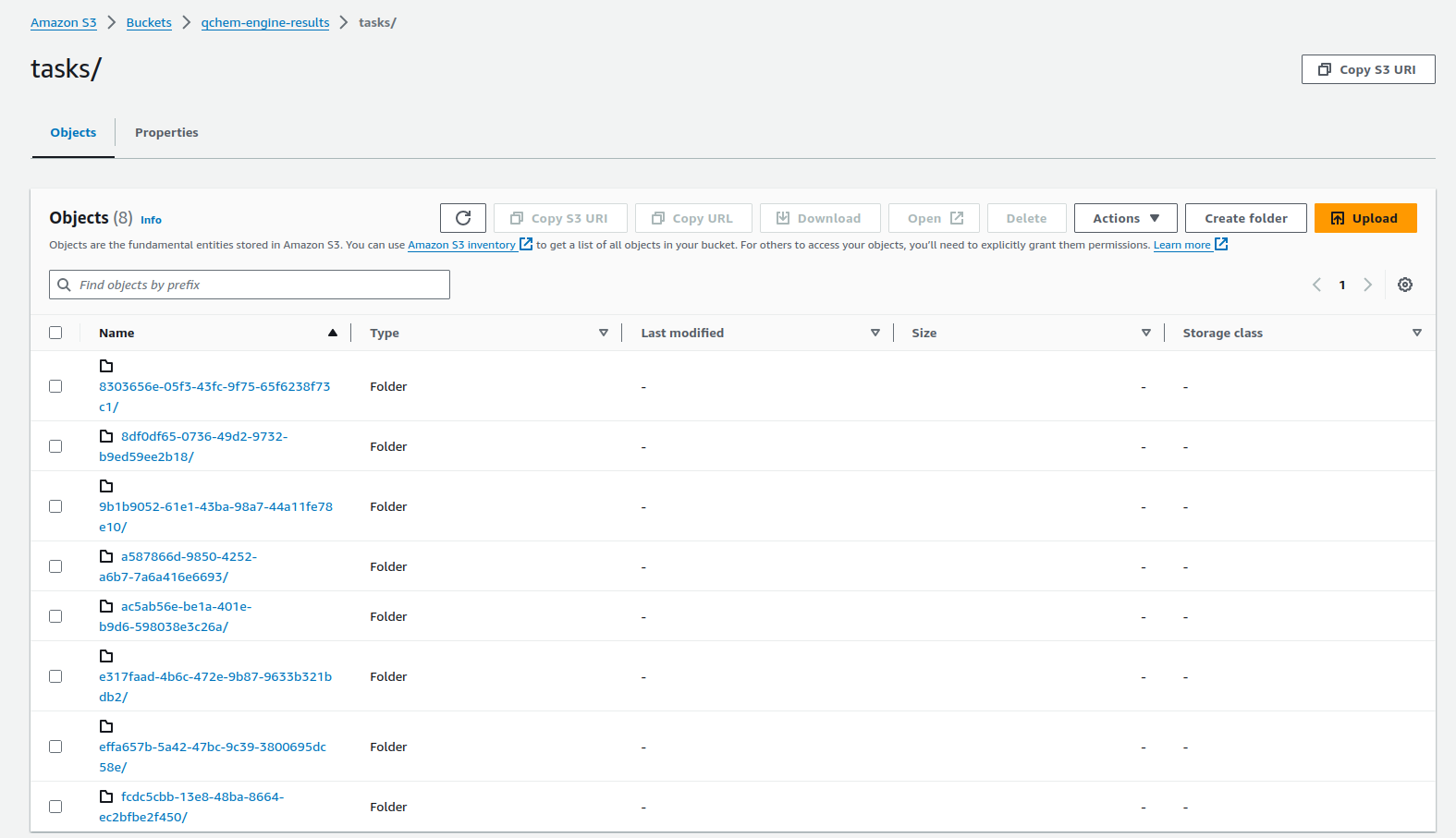Figure 5: S3 bucket view of all task folders for specific S3 bucket. The bucket name is defined by the user on the cloud provider platform of choice.

COSMO results data¶

You can get full access to all variables and parameters in the COSMO model. The results include for example:

the number of cosmo segments and their coordinates
the molecular surface area
the molecular COSMO volume
the cosmo surface charges for each segment

When retrieving the results of your calculation tasks you can get a complete and extensive overview which data is currently retrievable from the high performance COSMO implementation.

How to send off a task for a COSMO and sigma-profiles calculation via the Python SDK¶

Cebule SDK TaskType: COSMO¶

Performs COSMO (COnductor-like Screening MOdel) solvation calculations to model molecule-solvent interactions
Inputs:
geometry: List[float] - List of 3D coordinates in Angstrom (flattened x,y,z format)
symbols: List[str] - List of chemical element symbols for each atom
method: str - Quantum chemistry method (e.g., "SCF", "DFT")
basis: str - Basis set (e.g., "6-31g**")
dielec: float - Dielectric constant of the solvent (e.g., 78.0 for water, 1e6 to simulate a perfect conductor for COSMO-RS/SAC)
radius: List[float] - Van der Waals radii for each atom in Angstrom
Optional: optimize: bool - Whether to perform geometry optimization (default: False)
Optional: driver_convergence: str - Convergence criteria for geometry optimization (e.g., "loose", "default")
Optional: dft_energy_convergence: float - Energy convergence threshold for DFT calculations (default: 1e-7)
Cebule max_processors: Used to limit concurrency of quantum calculations
Output: Dictionary containing COSMO surface charge density and geometry.

Example:

from dotenv import load_dotenv
import mqsdk
from mqsdk.core.cebule import TaskType
import os

# Initialize the SDK with user credentials
load_dotenv()
session = mqsdk.Cebule(os.environ['EMAIL'], os.environ['PASSWORD'])

input_data = {
    "geometry": [
        0.0,  0.0000, -0.1294,
        0.0, -1.4941,  1.0274,
        0.0,  1.4941,  1.0274
        ],
    "symbols": ["O", "H", "H"],
    "method": "SCF",
    "basis": "6-31g**",
    "dielec": 78.0,
    "radius": [1.40, 1.16, 1.16],
    "optimize": True,
    "driver_convergence": "loose",
    "dft_energy_convergence": 1e-5
    }
task = session.cebule.create_task("COSMO Water Test", TaskType.COSMO,
                              input_data, nprocs=16)

# Result will contain COSMO surface charges and other information in a dictionary.

The COSMO task can also be connected to a previous GEOMETRY_OPT task to use optimized structures:

geometry_task_water = session.cebule.create_task("Geometry Opt water",
                            TaskType.GEOMETRY_OPT, 
                            smiles_list=["O"], 
                            force_field="mmff94",
                            optimization_method="g_xtb",
                            max_processors=4)

# The connected_task_id automatically uses the geometry from the geometry optimization task
cosmo_task_water = session.cebule.create_task("cosmo water", TaskType.COSMO,
    connected_task_id=geometry_task_water.id,
    method="dft",
    basis="def2-tzvp",
    dielec=1e6, # Simulate perfect conductor
    optimize=False,
    driver_convergence="loose",
    xc="becke88 perdew86",
    disp="vdw 4",
    dft_energy_convergence=1e-7,
    max_processors=64)

Find the whole Jupyter notebook under the following link: https://gitlab.com/mqsdk/python-sdk/-/blob/main/notebooks/2_COSMO_task_Cebule.ipynb

%# References

%[] "Atomistic Molecular Dynamics Simulation and COSMO-SAC Approach for Enhanced 1,3-Propanediol Extraction with Imidazolium-Based Ionic Liquids" https://doi.org/10.21203/rs.3.rs-3852183/v1

%[] "Phase equilibrium modeling of mixtures containing conformationally flexible molecules with the COSMO-SAC model" https://www.sciencedirect.com/science/article/abs/pii/S0167732222004342

%[] "Combination of molecular dynamics simulation, COSMO-RS, and experimental study to understand extraction of naphthenic acid" https://doi.org/10.1016/j.seppur.2021.119810

%[] "Combining Molecular Dynamics and Machine Learning to Predict Self-Solvation Free Energies and Limiting Activity Coefficients" https://doi.org/10.1021/acs.jcim.0c00479

%[] "Measurement of the solubility and density of the saturated solution of 3-aminophenol in different pure solvents from 283.1 to 323.1 K: Correlative to pure predictive thermodynamic modeling and %molecular dynamic simulation" https://doi.org/10.1016/j.molliq.2023.123478

%[] "Quantum chemical calculation, molecular dynamics simulation and process design for separation of heptane - butanol using ionic liquids extraction" https://doi.org/10.1016/j.molliq.2020.113851 -->

Openstax - chemistry 2e, 10.4 phase diagrams. \url https://openstax.org/books/chemistry-2e/pages/10-4-phase-diagrams. Accessed: 2024-10-27. ↩
John David Jackson. Classical electrodynamics. Wiley, 3rd ed. edition, 1999. ISBN 9780471309321. ↩
Jacopo Tomasi, Benedetta Mennucci, and Roberto Cammi. Quantum mechanical continuum solvation models. Chemical Reviews, 105(8):2999–3094, 2005. doi:10.1021/cr9904009. ↩↩
A. Klamt, C. Moya, and J. Palomar. A comprehensive comparison of the iefpcm and ss(v)pe continuum solvation methods with the cosmo approach. Journal of Chemical Theory and Computation, 11(9):4220–4225, 2015. doi:10.1021/acs.jctc.5b00601. ↩↩↩
W. Hackbusch. Integral equations :. Volume 120. Birkhäuser,, 1995. ISBN 0817628711, 3764328711, 9780817628710, 9783764328719. ↩