Chemical Reaction Networks Analysis

Overview

Chemical reaction networks have numerous different pathways to produce target molecules of interest. Solving the constrained combinatorial optimization problem of finding optimal reaction pathways has critical applications in synthesis planning and metabolic pathway analysis. This problem is generally a NP-hard problem due to the combinatorial explosion from the network graph size.

Mathematical Formulation

A chemical reaction network (CRN) can be represented as a bipartite directed graph with two types of nodes: reactions and species.

Each reaction in the network has associated costs:

• Unit cost (unit_cost): Cost per quantity of the reaction (e.g., substrate purchase, byproduct disposal)
• Fixed cost (fixed_cost): One-time cost incurred if the reaction occurs at all (e.g., equipment preparation)
• Bounds: Lower (low) and upper (high) limits on reaction quantities

The optimization problem, as presented by Mizuno and Komatsuzaki, can be formulated as:

minimize: Σ(r∈R) [c_r^unit × x_r + c_r^fixed × p(x_r)]

subject to: 
  ∀s∈S: Σ(r∈R) v_{s,r} × x_r = 0  (mass balance)
  ∀r∈R: l_r ≤ x_r ≤ u_r           (reaction bounds)

Where:

• R is the set of reactions, S is the set of species
• x_r is the quantity of reaction r (optimization variable)
• v_{s,r} is the signed stoichiometric coefficient of species s in reaction r
• p(x_r) is the positivity indicator function (1 if x_r > 0, 0 otherwise)

Task Types

RXN_NETWORK_OPT

• Optimize chemical reaction network pathways to minimize total cost while satisfying mass balance constraints
• Inputs: crn_data: Dict[str, List[Dict]] containing the reaction network definition with keys reaction_list and species_list, time_limit: int maximum solve time in seconds
• Cebule max_processors: Specify the number of cores to use
• Output: Dict[str, Union[Dict[str, int], float, bool, Dict[str, float]]] containing the keys reaction_quantities (mapping reaction names to optimal quantities), total_cost (minimum total cost achieved), solve_time (total time taken in seconds), and optimal (whether optimal solution was found)

Input Format

Within crn_data dictionary:

• reaction_list: Array of reaction definitions
• name: Unique identifier for the reaction
• fixed_cost: One-time cost if reaction occurs (≥0)
• unit_cost: Cost per unit quantity of reaction (≥0)
• low: Minimum allowed reaction quantity (≥0)
• high: Maximum allowed reaction quantity (≥low)
• species_list: Array of chemical species definitions
• name: Unique identifier for the species
• stoich: Dictionary mapping reaction names to signed stoichiometric coefficients
  • Positive values: species is produced by the reaction
  • Negative values: species is consumed by the reaction

Inflow and Outflow Reactions

Chemical reaction networks require boundary conditions to represent material inputs and product outputs. These are typically modeled as special reactions:

• Inflow reactions: Represent external material supply (e.g., raw material purchases). These reactions have no reactants and produce species needed by the network. They should positive low bounds if the material is a required input to ensure minimum supply, but if the material is optional (ex. one pathway to produce the desired target includes it but not another) a positive lower bound should not be given.

• Outflow reactions: Represent product extraction or waste disposal. These reactions consume species produced by the network and have no products. They may have positive low bounds to ensure minimum production targets are met. For species that require waste disposal (are byproducts or reactions but not required target chemicals) they should not have a positive lower bound.

Without inflow and outflow reactions, the mass balance constraints would force all reaction quantities to zero, as no net production or consumption would be possible in a closed system.

Example: Complete Solvay Process CRN

The following example details the Solvay Process CRN, shown in the below figure: 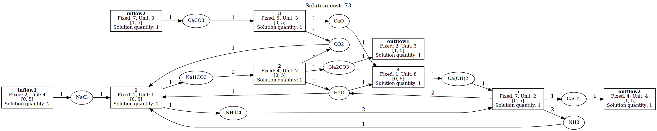Figure 1: Solvay Reaction Network with Optimal Solution Quantities

The input crn_data would be in the below format:

{
  "reaction_list": [
    {
      "name": "inflow1",
      "fixed_cost": 2,
      "unit_cost": 4,
      "low": 0,
      "high": 5
    },
    {
      "name": "inflow2",
      "fixed_cost": 7,
      "unit_cost": 3,
      "low": 1,
      "high": 5
    },
    {
      "name": "1",
      "fixed_cost": 2,
      "unit_cost": 1,
      "low": 0,
      "high": 5
    },
    {
      "name": "2",
      "fixed_cost": 4,
      "unit_cost": 2,
      "low": 0,
      "high": 5
    },
    {
      "name": "3",
      "fixed_cost": 9,
      "unit_cost": 3,
      "low": 0,
      "high": 5
    },
    {
      "name": "4",
      "fixed_cost": 1,
      "unit_cost": 8,
      "low": 0,
      "high": 5
    },
    {
      "name": "5",
      "fixed_cost": 7,
      "unit_cost": 2,
      "low": 0,
      "high": 5
    },
    {
      "name": "outflow1",
      "fixed_cost": 2,
      "unit_cost": 3,
      "low": 1,
      "high": 5
    },
    {
      "name": "outflow2",
      "fixed_cost": 4,
      "unit_cost": 4,
      "low": 1,
      "high": 5
    }
  ],
  "species_list": [
    {
      "name": "NaCl",
      "stoich": {
        "inflow1": 1,
        "1": -1
      }
    },
    {
      "name": "CO2",
      "stoich": {
        "1": -1,
        "2": 1,
        "3": 1
      }
    },
    {
      "name": "NaHCO3",
      "stoich": {
        "1": 1,
        "2": -2
      }
    },
    {
      "name": "Na2CO3",
      "stoich": {
        "2": 1,
        "outflow1": -1
      }
    },
    {
      "name": "H2O",
      "stoich": {
        "1": -1,
        "2": 1,
        "4": -1,
        "5": 2
      }
    },
    {
      "name": "NH3",
      "stoich": {
        "1": -1,
        "5": 2
      }
    },
    {
      "name": "NH4Cl",
      "stoich": {
        "1": 1,
        "5": -2
      }
    },
    {
      "name": "CaCO3",
      "stoich": {
        "inflow2": 1,
        "3": -1
      }
    },
    {
      "name": "CaO",
      "stoich": {
        "3": 1,
        "4": -1
      }
    },
    {
      "name": "Ca(OH)2",
      "stoich": {
        "4": 1,
        "5": -1
      }
    },
    {
      "name": "CaCl2",
      "stoich": {
        "5": 1,
        "outflow2": -1
      }
    }
  ]
}

This represents the complete Solvay process with:

• inflow1: NaCl supply (salt input)
• inflow2: CaCO₃ supply (limestone input)
• Reaction 1: Main ammonia-soda reaction: NaCl + CO₂ + H₂O + NH₃ → NaHCO₃ + NH₄Cl
• Reaction 2: Sodium carbonate formation: 2 NaHCO₃ → Na₂CO₃ + CO₂ + H₂O
• Reaction 3: Limestone calcination: CaCO₃ → CaO + CO₂
• Reaction 4: Lime slaking: CaO + H₂O → Ca(OH)₂
• Reaction 5: Ammonia recovery: Ca(OH)₂ + 2 NH₄Cl → 2 NH₃ + 2 H₂O + CaCl₂
• outflow1: Na₂CO₃ product extraction
• outflow2: CaCl₂ byproduct removal

Optimize reaction network with Cebule

# Create CRN optimization task
task_crn_opt = session.cebule.create_task(
    "Solvay Process Optimization",
    TaskType.RXN_NETWORK_OPT,
    crn_data=solvay_crn,
    time_limit=10
)

# Wait for result
result = session.cebule.wait_for_result(task_crn_opt.id, "result")
print(f"Optimal cost: {result['total_cost']}")
print(f"Reaction quantities: {result['reaction_quantities']}")
print(f"Optimization completed in {result['solve_time']} seconds")
print(f"Optimal solution found: {result['optimal']}")