Chemical Reaction Networks Analysis and Catalyst Design
Reaction Networks
Chemical reaction networks have numerous different pathways to produce target molecules of interest. Solving the constrained combinatorial optimization problem of finding optimal reaction pathways has critical applications in synthesis planning and metabolic pathway analysis. This problem is generally a NP-hard problem due to the combinatorial explosion from the network graph size. A pre-print publication published by us, MQS, presents a benchmark between different solvers for reaction network analysis and the CP-SAT based approach has been implemented in the Cebule SDK which shows almost the same performance with respect to computational time (identical optimal minimum) in comparison to the best performing solver (Gurobi).
Mathematical Formulation
A chemical reaction network (CRN) can be represented as a bipartite directed graph with two types of nodes: reactions and species.
Each reaction in the network has associated costs:
- Unit cost (
unit_cost): Cost per quantity of the reaction (e.g., substrate purchase, byproduct disposal) - Fixed cost (
fixed_cost): One-time cost incurred if the reaction occurs at all (e.g., equipment preparation) - Bounds: Lower (
low) and upper (high) limits on reaction quantities
The optimization problem, as presented by Mizuno and Komatsuzaki, can be formulated as:
minimize: Σ(r∈R) [c_r^unit × x_r + c_r^fixed × p(x_r)]

subject to:
  ∀s∈S: Σ(r∈R) v_{s,r} × x_r = 0  (mass balance)
  ∀r∈R: l_r ≤ x_r ≤ u_r           (reaction bounds)
Where:
Ris the set of reactions,Sis the set of speciesx_ris the quantity of reaction r (optimization variable)v_{s,r}is the signed stoichiometric coefficient of species s in reaction rp(x_r)is the positivity indicator function (1 if x_r > 0, 0 otherwise)
Task Types
RXN_OPT
- Optimize chemical reaction network pathways to minimize total cost while satisfying mass balance constraints
- Inputs:
crn_data: Dict[str, List[Dict]]containing the reaction network definition with keysreaction_listandspecies_list,time_limit: intmaximum solve time in seconds - Cebule max_processors: Specify the number of cores to use
- Output:
Dict[str, Union[Dict[str, int], float, bool, Dict[str, float]]]containing the keysreaction_quantities(mapping reaction names to optimal quantities),total_cost(minimum total cost achieved),solve_time(total time taken in seconds), andoptimal(whether optimal solution was found)
Input Format
Within crn_data dictionary:
reaction_list: Array of reaction definitionsname: Unique identifier for the reactionfixed_cost: One-time cost if reaction occurs (≥0)unit_cost: Cost per unit quantity of reaction (≥0)low: Minimum allowed reaction quantity (≥0)high: Maximum allowed reaction quantity (≥low)species_list: Array of chemical species definitionsname: Unique identifier for the speciesstoich: Dictionary mapping reaction names to signed stoichiometric coefficients- Positive values: species is produced by the reaction
- Negative values: species is consumed by the reaction
Inflow and Outflow Reactions
Chemical reaction networks require boundary conditions to represent material inputs and product outputs. These are typically modeled as special reactions:
-
Inflow reactions: Represent external material supply (e.g., raw material purchases). These reactions have no reactants and produce species needed by the network. They should positive
lowbounds if the material is a required input to ensure minimum supply, but if the material is optional (ex. one pathway to produce the desired target includes it but not another) a positive lower bound should not be given. -
Outflow reactions: Represent product extraction or waste disposal. These reactions consume species produced by the network and have no products. They may have positive
lowbounds to ensure minimum production targets are met. For species that require waste disposal (are byproducts or reactions but not required target chemicals) they should not have a positive lower bound.
Without inflow and outflow reactions, the mass balance constraints would force all reaction quantities to zero, as no net production or consumption would be possible in a closed system.
Example: Complete Solvay Process CRN
The following example details the Solvay Process CRN, shown in the below figure:
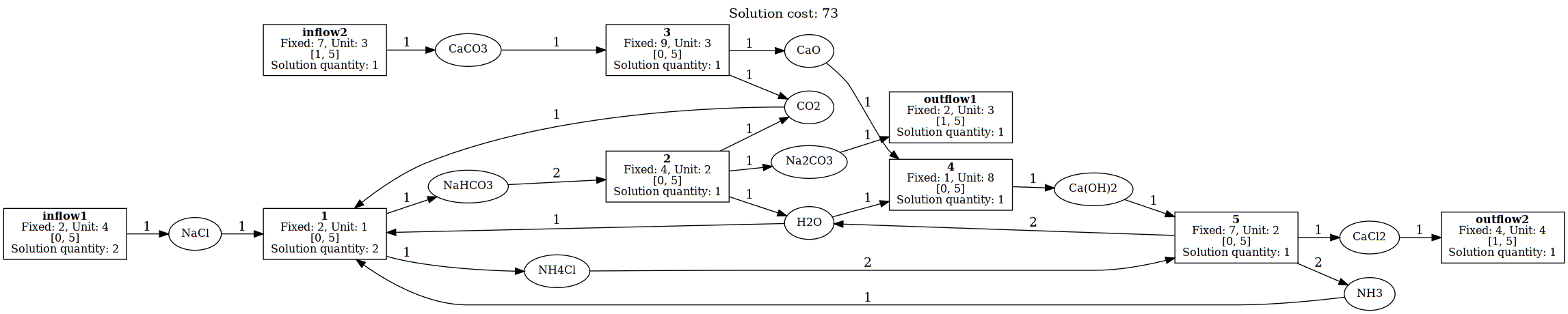 Figure 1: Solvay Reaction Network with Optimal Solution Quantities
The input crn_data would be in the below format:
{
  "reaction_list": [
    {
      "name": "inflow1",
      "fixed_cost": 2,
      "unit_cost": 4,
      "low": 0,
      "high": 5
    },
    {
      "name": "inflow2",
      "fixed_cost": 7,
      "unit_cost": 3,
      "low": 1,
      "high": 5
    },
    {
      "name": "1",
      "fixed_cost": 2,
      "unit_cost": 1,
      "low": 0,
      "high": 5
    },
    {
      "name": "2",
      "fixed_cost": 4,
      "unit_cost": 2,
      "low": 0,
      "high": 5
    },
    {
      "name": "3",
      "fixed_cost": 9,
      "unit_cost": 3,
      "low": 0,
      "high": 5
    },
    {
      "name": "4",
      "fixed_cost": 1,
      "unit_cost": 8,
      "low": 0,
      "high": 5
    },
    {
      "name": "5",
      "fixed_cost": 7,
      "unit_cost": 2,
      "low": 0,
      "high": 5
    },
    {
      "name": "outflow1",
      "fixed_cost": 2,
      "unit_cost": 3,
      "low": 1,
      "high": 5
    },
    {
      "name": "outflow2",
      "fixed_cost": 4,
      "unit_cost": 4,
      "low": 1,
      "high": 5
    }
  ],
  "species_list": [
    {
      "name": "NaCl",
      "stoich": {
        "inflow1": 1,
        "1": -1
      }
    },
    {
      "name": "CO2",
      "stoich": {
        "1": -1,
        "2": 1,
        "3": 1
      }
    },
    {
      "name": "NaHCO3",
      "stoich": {
        "1": 1,
        "2": -2
      }
    },
    {
      "name": "Na2CO3",
      "stoich": {
        "2": 1,
        "outflow1": -1
      }
    },
    {
      "name": "H2O",
      "stoich": {
        "1": -1,
        "2": 1,
        "4": -1,
        "5": 2
      }
    },
    {
      "name": "NH3",
      "stoich": {
        "1": -1,
        "5": 2
      }
    },
    {
      "name": "NH4Cl",
      "stoich": {
        "1": 1,
        "5": -2
      }
    },
    {
      "name": "CaCO3",
      "stoich": {
        "inflow2": 1,
        "3": -1
      }
    },
    {
      "name": "CaO",
      "stoich": {
        "3": 1,
        "4": -1
      }
    },
    {
      "name": "Ca(OH)2",
      "stoich": {
        "4": 1,
        "5": -1
      }
    },
    {
      "name": "CaCl2",
      "stoich": {
        "5": 1,
        "outflow2": -1
      }
    }
  ]
}
This represents the complete Solvay process with:
- inflow1: NaCl supply (salt input)
- inflow2: CaCO₃ supply (limestone input)
- Reaction 1: Main ammonia-soda reaction: NaCl + CO₂ + H₂O + NH₃ → NaHCO₃ + NH₄Cl
- Reaction 2: Sodium carbonate formation: 2 NaHCO₃ → Na₂CO₃ + CO₂ + H₂O
- Reaction 3: Limestone calcination: CaCO₃ → CaO + CO₂
- Reaction 4: Lime slaking: CaO + H₂O → Ca(OH)₂
- Reaction 5: Ammonia recovery: Ca(OH)₂ + 2 NH₄Cl → 2 NH₃ + 2 H₂O + CaCl₂
- outflow1: Na₂CO₃ product extraction
- outflow2: CaCl₂ byproduct removal
Optimize reaction network with Cebule
# Create CRN optimization task
task_crn_opt = session.cebule.create_task(
    "Solvay Process Optimization",
    TaskType.RXN_NETWORK_OPT,
    crn_data=solvay_crn,
    time_limit=10
)

# Wait for result
result = session.cebule.wait_for_result(task_crn_opt.id, "result")
print(f"Optimal cost: {result['total_cost']}")
print(f"Reaction quantities: {result['reaction_quantities']}")
print(f"Optimization completed in {result['solve_time']} seconds")
print(f"Optimal solution found: {result['optimal']}")
Catalyst Design
Overview
The Catalyst Design module provides a comprehensive computational framework for designing and optimizing heterogeneous catalysts for chemical reactions. By combining quantum mechanical calculations with machine learning, the module enables:
- High-throughput screening of bimetallic alloy surfaces
- MLIP models wrapper and benchmarking to assess which machine learned interatomic potential model provides best results
- Turnover Frequency (TOF) prediction using microkinetic modeling
- Generative design of novel catalyst compositions using Generative Adversarial Networks (GANs)
- Surface energy analysis through Wulff construction
The workflow follows an iterative optimization loop where catalyst candidates are generated, evaluated computationally, and refined through machine learning to discover high-performance materials.
Theoretical Background
Surface Reactions and Turnover Frequency
Heterogeneous catalysis occurs at the interface between a solid catalyst surface and gas-phase reactants. The catalytic activity is quantified by the Turnover Frequency (TOF), which represents the number of reaction cycles per active site per second.
The TOF depends on:
- Reaction energies (ΔE): Energy differences between reactants and products for each elementary step
- Activation barriers (Eₐ): Energy barriers that must be overcome for reactions to proceed
- Surface coverages (θ): Fraction of surface sites occupied by each adsorbate species
- Temperature (T) and Pressure (P): Thermodynamic conditions
Brønsted-Evans-Polanyi (BEP) Relation
Activation barriers are estimated using the BEP relation, which correlates the activation energy with the reaction energy:
Where α and β are universal scaling parameters. For stepped transition metal surfaces 1: - α = 0.87 - β = 1.34 eV
Reaction Network Format
Reaction networks are defined in plain text files using the following syntax:
# Comment lines start with #
MOLECULE1 + 2*surf    --ER-->  2*ATOM1_fcc
MOLECUEL2 + 2*surf    --ER-->  2*ATOM2_bridge
MOLECULE3_ontop       --ads--> MOLECULE3 + surf
Syntax elements:
-
species_site: Adsorbate species at a specific surface site (e.g.,ATOM1_fcc,ATOM2_bridge) -
surf: Represents a vacant surface site -
n*species: Stoichiometric coefficient (e.g.,2*ATOM1_fcc) -
--ER-->: Eley-Rideal mechanism (gas-surface reaction) -
--ads-->: Adsorption/desorption step
Supported adsorption sites: ontop, bridge, fcc, hcp, 3fold, 4fold
Supported Energy Calculators (includes MLIP, tight-binding and PW-DFT models)
| Calculator | Description |
|---|---|
mace-mp |
MACE-MP machine learning potential |
orb |
ORB machine learning potential |
pet-mad |
PET-MAD potential |
grace-2l-omat |
GRACE-2L potential |
tblite |
GFN-xTB tight-binding DFT |
pw-dft |
Plane-wave DFT |
Task Types
MAKE_SURF
Generates a dataset of bimetallic alloy surfaces with randomized compositions.
Description: Creates catalyst surface structures by substituting atoms of a primary element with a secondary element at random positions. The surfaces can be FCC, stepped FCC (211), or stepped HCP structures, optionally with support materials.
Inputs:
| Parameter | Type | Required | Default | Description |
|---|---|---|---|---|
element1 |
str |
Yes | - | Primary element symbol (e.g., "Ru", "Pt") |
element2 |
str |
Yes | - | Secondary element for alloying |
surface_type |
str |
No | "step_fcc" |
Surface structure: "fcc", "step_fcc", or "step_hcp" |
n_surfaces |
int |
No | 1 | Number of unique surfaces to generate |
lattice_const |
float |
Yes | - | Lattice constant of primary element [Å] |
vacuum |
float |
No | 10.0 | Vacuum layer thickness [Å] |
supercell_size_x |
int |
No | 3 | Supercell repetitions in x-direction |
supercell_size_y |
int |
No | 4 | Supercell repetitions in y-direction |
layers |
int |
No | 3 | Number of atomic layers |
layers_to_fix |
int |
No | 1 | Bottom layers fixed during optimization |
reaction_network |
dict |
Yes | - | Reaction network definition |
dataset_tag |
str |
Yes | - | Unique identifier for the dataset |
Optional Support Parameters:
| Parameter | Type | Description |
|---|---|---|
support |
str |
Support material formula (e.g., "OCeO" for ceria) |
support_structure |
str |
Crystal structure: "fcc", "fluorite", "rocksalt", etc. |
support_lattice_const |
float |
Support lattice constant [Å] |
n_support_layers |
int |
Number of support layers |
support_supercell_size_x |
int |
Support supercell size in x |
support_supercell_size_y |
int |
Support supercell size in y |
Output:
surf_config = {
    "surface_type": "step_fcc",
    "symbol": "ATOM1",
    "symbol2": "ATOM2",
    "vac": 10.0,
    "lattice_const": 2.7,
    "lateral_supercell_size": [3, 4],
    "nlayer": 3,
    "support_name": None,
    "support_lattice_const": None,
    "support_structure": None,
    "support_lateral_supercell_size": None,
    "support_nlayer": None,
    "layers_to_fix": 1,
}
Example with Cebule SDK:
from cebule import TaskType

# Create surface generation task
task_make_surf = session.cebule.create_task(
    "Generate ATOM1ATOM2 alloy surfaces",
    TaskType.MAKE_SURF,
    element1="ATOM1",
    element2="ATOM2",
    surface_type="step_fcc",
    n_surfaces=100,
    lattice_const=2.7,
    vacuum=10.0,
    layers=3,
    reaction_network=XY_network,
    dataset_tag="runi_screening_v1"
)

result = session.cebule.wait_for_result(task_make_surf.id, "result")
print(f"Generated {result['n_surfaces']} surface configurations")
GAS_SPECIES_ENERGY
Calculates reference energies for gas-phase species involved in the reaction network.
Description: Computes optimized geometries and total energies for all gas-phase molecules referenced in the reaction network. These serve as reference energies for computing adsorption and reaction energies.
Inputs:
| Parameter | Type | Required | Default | Description |
|---|---|---|---|---|
energy_calculator |
str |
Yes | - | Calculator type (see supported calculators) |
optimizer_type |
str |
No | "fire" |
Geometry optimizer: "fire", "lbfgs", "gpmin" |
unitcell_length |
float |
No | 12.0 | Cubic unit cell size for gas molecules [Å] |
temperature |
float |
No | 700.0 | Temperature for thermodynamic corrections [K] |
pressure |
float |
No | 100.0 | Total pressure [bar] |
dataset_tag |
str |
No | - | Associate results with a dataset |
num_cores |
int |
No | All | Number of CPU cores to use |
Output:
reaction_energies_gas = {
    "MOLECULE1": -16.45,   # Energy in eV
    "MOLECULE2": -6.77,
    "MOLECULE3": -19.82,
}
Example:
task_gas = session.cebule.create_task(
    "Calculate gas phase energies",
    TaskType.GAS_SPECIES_ENERGY,
    energy_calculator="mace-mp",
    temperature=700.0,
    pressure=100.0,
    dataset_tag="run_screening_1"
)

gas_energies = session.cebule.wait_for_result(task_gas.id, "result")
SURFACE_REACTION_ENERGIES
Calculates adsorption and reaction energies for all surfaces in a dataset.
Description: For each surface structure in the dataset, computes the energies of all adsorbate configurations defined in the reaction network, then calculates reaction energies (ΔE) for each elementary step.
Inputs:
| Parameter | Type | Required | Default | Description |
|---|---|---|---|---|
reaction_type |
dict |
Yes | - | Reaction network definition |
temperature |
float |
No | 700.0 | Reaction temperature [K] |
pressure |
float |
No | 100.0 | Total pressure [bar] |
adsorbate_positions |
dict |
No | - | Override automatic adsorbate placement |
backup_site |
list |
No | - | Fallback sites if primary fails |
uncertainty |
bool |
No | False |
Enable ensemble uncertainty quantification |
fmax |
float |
No | 0.05 | Max force for geometry optimization [eV/Å] |
dataset_tag |
str |
Yes | - | Dataset to process |
num_cores |
int |
No | All | Number of CPU cores |
For tblite calculator only:
| Parameter | Type | Default | Description |
|---|---|---|---|
gfn |
int |
2 | GFN version (1 or 2) |
electronic_temperature |
float |
300.0 | SCF smearing temperature [K] |
geometry_opt |
bool |
False |
Refine with PW-DFT after tblite |
Output:
reaction_energies_surf = {
    "surf_001": {
        "reaction_1": -0.82,  # dissociation ΔE [eV]
        "reaction_2": -0.45,  # dissociation
        "reaction_3": 0.12,   # Reaction 3
        "reaction_4": -0.23,  # Reaction 4
        "reaction_5": -0.15,  # Reaction 5
        "reaction_6": 0.67,   # Reaction 6
    },
    # ... additional surfaces
}
Example:
task_energies = session.cebule.create_task(
    "Calculate surface reaction energies",
    TaskType.SURFACE_REACTION_ENERGIES,
    reaction_type=reaction_network,
    temperature=400.0,
    pressure=50.0,
    uncertainty=True, # Enable kinetic uncertainty
    dataset_tag="run_screening_1"
)

# This task may take significant time for large datasets
result = session.cebule.wait_for_result(task_energies.id, "result", timeout=3600)
GAN_TOF
Trains a Generative Adversarial Network to discover high-performance catalyst compositions.
Description: Uses computed TOF values to train a conditional GAN that learns the relationship between atomic composition and catalytic activity. The generator produces new catalyst compositions optimized for the highest TOF class.
Inputs:
| Parameter | Type | Required | Default | Description |
|---|---|---|---|---|
reaction_type |
dict/str |
Yes | - | Reaction network or tag reference |
dataset_tag |
str |
Yes | - | Dataset with computed TOF values |
epochs |
int |
No | 2000 | Training epochs |
nclass |
int |
No | 5 | Number of TOF classes for conditioning |
score_max |
float |
No | 5.0 | Upper TOF outlier threshold (log₁₀ scale) |
score_min |
float |
No | -17.0 | Lower TOF outlier threshold (log₁₀ scale) |
scaler |
str |
No | "standard" |
Data scaling: "standard" or "minmax" |
min_loss_diff |
float |
No | 1.0 | Minimum G_loss - D_loss for successful training |
Output:
surf_data = {
    "surfaces": [
        {
            "chemical_formula": "ATOMxATOMy",
            "atomic_numbers": [44, 44, 28, 44, ...],  # Per-atom composition
            "run": 3,  # GAN iteration number
        },
        # ... additional generated surfaces
    ],
    "training_loss": {
        "D_loss": [1.2, 0.8, 0.5, ...],
        "G_loss": [2.1, 1.5, 1.2, ...],
    }
}
Example:
# Run GAN optimization
task_gan = session.cebule.create_task(
    "GAN catalyst optimization",
    TaskType.GAN_TOF,
    reaction_type=reaction_network,
    dataset_tag="run_screening_1",
    epochs=3000,
    nclass=5,
    scaler="standard"
)

result = session.cebule.wait_for_result(task_gan.id, "result")
print(f"Generated {len(result['surfaces'])} new catalyst candidates")

# The new surfaces are automatically added to the dataset
# Run SURFACE_REACTION_ENERGIES again to evaluate them
Training Tips:
-
Dataset size: Minimum ~80 surfaces recommended for effective training
-
Class balance: Ensure reasonable distribution across TOF classes
-
Convergence: Monitor that G_loss - D_loss > min_loss_diff
-
Iteration: Repeat GAN → Energy calculation cycle until TOF converges
WULFF_CONSTRUCTION
Computes equilibrium crystal shape and surface energies using Wulff construction.
Description: Determines the thermodynamically stable crystal shape by calculating surface energies for all low-index Miller planes and constructing the Wulff shape. Optionally includes adsorbate effects on surface stability.
flowchart TD
    A[Generate all slabs up to Miller index 3] --> B

    subgraph loop["For each Miller index (hkl)"]
        B[Initialize N = 10 layers]
        B --> C[Compute slab energy E_slab]
        C --> D[Calculate surface energy γ = E_slab - N×E_bulk / 2A]
        D --> E{Adsorbate?}
        E -->|Yes| F[Add adsorbate, compute γ_ads]
        E -->|No| G[γ_final = γ]
        F --> G
        G --> H{Converged?<br/>Δγ ≤ 0.005 eV/Ų}
        H -->|No| I[N = N + 1]
        I --> C
        H -->|Yes| J[Record γ and hkl]
    end

    J --> K[Build Wulff polyhedron]
    K --> L[Output surface areas and energies]
Inputs:
| Parameter | Type | Required | Default | Description |
|---|---|---|---|---|
bulk |
str |
Yes | - | Element symbol for bulk structure |
bulk_structure |
str |
Yes | - | Crystal structure: "fcc" or "hcp" |
energy_calculator |
str |
Yes | - | Calculator for energy evaluation |
reaction_type |
dict/str |
No | - | Include reaction network for TOF |
adsorbate |
str |
No | - | Adsorbate species to include |
site |
str |
No | - | Adsorption site (required if adsorbate set) |
dataset_tag |
str |
Yes | - | Output dataset identifier |
Optional Parameters:
| Parameter | Type | Default | Description |
|---|---|---|---|
gas_species |
str |
- | Gas molecule containing adsorbate |
extra_gas_mol |
str |
- | Additional gas reference |
extra_gas_scalar |
float |
- | Scaling for extra gas energy |
backup_site |
str |
- | Fallback adsorption site |
md |
bool |
False |
Use NVT MD for energy |
md_temperature |
float |
700.0 | MD temperature [K] |
pressure |
float |
- | Pressure for rate calculations [bar] |
min_slab_size |
float |
10.0 | Minimum slab thickness [Å] |
min_vacuum_size |
float |
18.0 | Minimum vacuum [Å] |
fmax |
float |
1000.0 | Max force (large = no optimization) |
compute_tof |
bool |
False |
Calculate TOF for each facet |
num_cores |
int |
All | CPU cores to use |
surface_hull_tol |
float |
1.5 | Tolerance for surface atom detection |
Output:
surf_energies = {
    "miller_indices": {
        (1, 1, 1): {
            "surface_energy": 0.092,  # eV/Ų
            "area_fraction": 0.45,
        },
        (1, 0, 0): {
            "surface_energy": 0.105,
            "area_fraction": 0.30,
        },
        (1, 1, 0): {
            "surface_energy": 0.098,
            "area_fraction": 0.25,
        },
    },
    "adsorption_energies": {  # If adsorbate specified
        (1, 1, 1): -0.82,
        (1, 0, 0): -0.75,
    },
    "tof_values": {  # If compute_tof=True
        (1, 1, 1): 1.2e-3,
        (1, 0, 0): 8.5e-4,
    },
    "activation_barriers": {
        (1, 1, 1): [0.87, 0.45, 0.92, 0.67, 0.55, 0.43],
    }
}
Example:
task_wulff = session.cebule.create_task(
    "Ru Wulff construction with N adsorbate",
    TaskType.WULFF_CONSTRUCTION,
    bulk="Atom1",
    bulk_structure="hcp",
    energy_calculator="mace-mp",
    adsorbate="Atom2",
    site="fcc",
    compute_tof=True,
    reaction_type=formation_network,
    dataset_tag="Atom2_wulff_analysis"
)

result = session.cebule.wait_for_result(task_wulff.id, "result")

# Access facet-specific information
for miller, data in result['miller_indices'].items():
    print(f"{miller}: γ = {data['surface_energy']:.3f} eV/Ų, "
          f"area = {data['area_fraction']*100:.1f}%")
VISUALIZE_SURF
Generates visualizations of catalyst surfaces with adsorbates.
Description: Creates 3D structural visualizations of catalyst surfaces, showing atomic positions, unit cells, and adsorbate configurations.
Inputs:
| Parameter | Type | Required | Default | Description |
|---|---|---|---|---|
catalyst_surface_tag |
str |
Yes | - | Dataset tag of surface to visualize |
reaction_type |
dict/str |
Yes | - | Reaction network definition |
adsorbate |
str |
No | - | Adsorbate to display |
site |
str |
No | - | Adsorption site (required with adsorbate) |
vacuum |
float |
No | 10.0 | Vacuum thickness [Å] |
show_unit_cell |
bool |
No | True |
Display unit cell boundaries |
adsorbate_positions |
dict |
No | - | Manual position override |
dataset_tag |
str |
Yes | - | Output identifier |
Output: ASE Atoms object compatible with ase.visualize.view().
Example:
task_vis = session.cebule.create_task(
    "Visualize best catalyst",
    TaskType.VISUALIZE_SURF,
    catalyst_surface_tag="surf_042",  # Best performing surface
    reaction_type=formation_network,
    adsorbate="MOLECULE2",
    site="bridge",
    show_unit_cell=True,
    dataset_tag="run_screening_1"
)

atoms = session.cebule.wait_for_result(task_vis.id, "result")

# Use ASE visualization
from ase.visualize import view
view(atoms)
GAN
Analyzes GAN training progress and catalyst improvement over iterations.
Description: Generates analysis plots showing how catalyst performance (TOF) evolves across GAN training iterations.
Inputs:
| Parameter | Type | Required | Default | Description |
|---|---|---|---|---|
reaction_type |
dict/str |
Yes | - | Reaction network |
dataset_tag |
str |
Yes | - | Dataset with GAN history |
target_metric |
str |
No | "TOF" |
Metric to track |
score_max |
float |
No | 5.0 | Upper outlier threshold |
score_min |
float |
No | -17.0 | Lower outlier threshold |
Output: - Data structure for plotting TOF vs. GAN iteration - PNG/bytes object for direct visualization
Example:
task_gan_analysis = session.cebule.create_task(
    "Analyze GAN optimization progress",
    TaskType.GAN,
    reaction_type=formation_network,
    dataset_tag="run_screening_1",
    target_metric="TOF"
)

result = session.cebule.wait_for_result(task_gan_analysis.id, "result")


# Plot shows TOF improvement over GAN iterations
import matplotlib.pyplot as plt
plt.figure(figsize=(10, 6))
plt.plot(result['iterations'], result['mean_tof'], 'b-', label='Mean TOF')
plt.fill_between(result['iterations'],
                 result['min_tof'], result['max_tof'],
                 alpha=0.3, label='TOF range')
plt.xlabel('GAN Iteration')
plt.ylabel('log10(TOF)')
plt.legend()
plt.savefig('gan_progress.png')
POTENTIAL_ENERGY
Generates potential energy diagrams for reaction pathways.
Description: Creates energy profile plots showing the energetics of each elementary step along the reaction coordinate.
Inputs:
| Parameter | Type | Required | Default | Description |
|---|---|---|---|---|
reaction_type |
dict/str |
Yes | - | Reaction network |
dataset_tag |
str |
Yes | - | Dataset with energy data |
Output: - Data structure with ΔE values for each reaction step - PNG/bytes object for the energy diagram
Example:
task_ped = session.cebule.create_task(
    "Generate potential energy diagram",
    TaskType.POTENTIAL_ENERGY,
    reaction_type=reaction_network,
    dataset_tag="run_screening_1"
)

result = session.cebule.wait_for_result(task_ped.id, "result")

# Result contains energy levels for each state along reaction path
print("Reaction energies [eV]:")
for step, energy in result['reaction_energies'].items():
    print(f"  {step}: ΔE = {energy:+.3f}")
FRACTIONAL_COVERAGES
Analyzes surface coverage distributions across multiple catalyst surfaces.
Description: Computes and compares the fractional surface coverages of all adsorbate species under reaction conditions for multiple catalyst surfaces.
Inputs:
| Parameter | Type | Required | Default | Description |
|---|---|---|---|---|
reaction_type |
dict/str |
Yes | - | Reaction network |
dataset_tag_list |
list |
Yes | - | List of dataset tags to compare |
Output: - Coverage data for each species on each surface - Visualization comparing coverage distributions
Example:
task_coverage = session.cebule.create_task(
    "Compare surface coverages",
    TaskType.FRACTIONAL_COVERAGES,
    reaction_type=nh3_formation_network,
    dataset_tag_list=["TAG1", "TAG2", "TAG3"]
)

result = session.cebule.wait_for_result(task_coverage.id, "result")

# Access coverage data
for dataset, coverages in result['coverages'].items():
    print(f"\n{dataset}:")
    for species, theta in coverages.items():
        print(f"  θ({species}) = {theta:.4f}")
REACTION_ENERGIES_COMPARISON
Compares reaction energies across different surfaces or calculation methods.
Description: Generates statistical comparisons of reaction energies, useful for validating computational methods or comparing catalyst families.
Inputs:
| Parameter | Type | Required | Default | Description |
|---|---|---|---|---|
reaction_type |
dict/str |
Yes | - | Reaction network |
dataset_tag |
str |
Yes | - | Dataset for comparison |
Output: - Statistical metrics (mean, max, min differences) for each reaction - Comparison visualization
Example:
task_compare = session.cebule.create_task(
    "Compare reaction energies across methods",
    TaskType.REACTION_ENERGIES_COMPARISON,
    reaction_type=reaction_network,
    dataset_tag="method_comparison_v1"
)

result = session.cebule.wait_for_result(task_compare.id, "result")

print("Reaction energy comparison:")
print(f"  Overall mean difference: {result['overall_mean']:.3f} eV")
print(f"  Overall max difference:  {result['overall_max']:.3f} eV")
print(f"  Overall min difference:  {result['overall_min']:.3f} eV")
Complete Workflow Example
The following example demonstrates a complete catalyst optimization workflow for a reaction network which can adapted:
from cebule import Session, TaskType

# Initialize session
session = Session()

# Define reaction network
reaction_network = {
    "name": "example_rx",
    "reactions": [
    "MOLECULE1 + 2*surf --ER-->  2*ATOM1_fcc",
        "MOLECUEL2 + 2*surf --ER-->  2*ATOM2_bridge",
        "MOLECULE3_ontop --ads--> MOLECULE3 + surf"
    ]
}

DATASET_TAG = "run_optimization_1"

# Step 1: Generate initial catalyst surfaces
task_surf = session.cebule.create_task(
    "Generate ATOM1ATOM2 surfaces",
    TaskType.MAKE_SURF,
    element1="ATOM1",
    element2="ATOM1",
    surface_type="step_fcc",
    n_surfaces=100,
    lattice_const=2.7,
    layers=3,
    reaction_network=reaction_network,
    dataset_tag=DATASET_TAG
)
session.cebule.wait_for_result(task_surf.id, "result")

# Step 2: Calculate gas-phase reference energies
task_gas = session.cebule.create_task(
    "Gas phase energies",
    TaskType.GAS_SPECIES_ENERGY,
    energy_calculator="mace-mp",
    temperature=700.0,
    pressure=100.0,
    dataset_tag=DATASET_TAG
)
session.cebule.wait_for_result(task_gas.id, "result")

# Iterative GAN optimization loop
for iteration in range(5):
    print(f"\n=== GAN Iteration {iteration + 1} ===")

    # Step 3: Calculate surface reaction energies
    task_energies = session.cebule.create_task(
        f"Surface energies (iter {iteration})",
        TaskType.SURFACE_REACTION_ENERGIES,
        reaction_type=reaction_network,
        temperature=700.0,
        pressure=100.0,
        dataset_tag=DATASET_TAG
    )
    session.cebule.wait_for_result(task_energies.id, "result", timeout=7200)

    # Step 4: Train GAN and generate new candidates
    task_gan = session.cebule.create_task(
        f"GAN training (iter {iteration})",
        TaskType.GAN_TOF,
        reaction_type=reaction_network,
        dataset_tag=DATASET_TAG,
        epochs=2000,
        nclass=5
    )
    result = session.cebule.wait_for_result(task_gan.id, "result")

    print(f"Generated {len(result.get('surfaces', []))} new candidates")

# Step 5: Generate final analysis
task_analysis = session.cebule.create_task(
    "Final GAN analysis",
    TaskType.GAN,
    reaction_type=reaction_network,
    dataset_tag=DATASET_TAG
)
analysis = session.cebule.wait_for_result(task_analysis.id, "result")

# Step 6: Visualize best catalyst
task_ped = session.cebule.create_task(
    "Energy diagram for best catalyst",
    TaskType.POTENTIAL_ENERGY,
    reaction_type=reaction_network,
    dataset_tag=DATASET_TAG
)
session.cebule.wait_for_result(task_ped.id, "result")

print("\nOptimization complete!")
print(f"Best TOF achieved: {analysis['best_tof']:.2e}")
print(f"Best composition: {analysis['best_composition']}")
-
J.K. Nørskov, T. Bligaard, A. Logadottir, S. Bahn, L.B. Hansen, M. Bollinger, H. Bengaard, B. Hammer, Z. Sljivancanin, M. Mavrikakis, Y. Xu, S. Dahl, and C.J.H. Jacobsen. Universality in heterogeneous catalysis. Journal of Catalysis, 209(2):275–278, 2002. doi:https://doi.org/10.1006/jcat.2002.3615. ↩