Quantum Computing

On this page we are going to present you the quantum computing methods we have developed and made available through our SDK:

• A mapping and measurement method for electronic structure problem formulations ¹

• A tensor networks based methodology to optimize an Hamiltonian for generating an optimized Hamiltonian to be solved on a classical computer (CPU, GPU) while at the same time generating an improved state with a quantum circuit (Ansatz) to be solved on a QPU. ²

• Active space selection methods

• Zero-noise extrapolation

• Quantum circuit generation methods such as our genetic evolution method in our Xenakis package

• Our open-source benchmarking framework to test different variational quantum algorithms (VQA) such as VQE, QAOA etc. and other methods (QSE, GQE, CP-SAT).

• Our research articles and research projects

A Cebule SDK task can be run in the following way:

# Import needed packages
from dotenv import load_dotenv
import json
import mqsdk
from mqsdk.core.cebule import TaskType
import os

# Initialize the SDK with user credentials
load_dotenv()
session = mqsdk.Cebule(os.environ['EMAIL'], os.environ['PASSWORD'])

# The input data specific to the individual task types
input_data = '''
{
    "geometry": [
        0.0, 0.0, -0.068,
        0.0, -0.791, 0.544,
        0.0, 0.791, 0.544
    ],
    "symbols": ["O", "H", "H"],
    ...
    ...
}
'''

# Run a task via Cebule SDK on the Cebule HPC
task = session.cebule.create_task("Your title for the specific task run", TaskType.MOL_MAP, input_data)

For more information about the Cebule SDK: https://gitlab.com/mqsdk/python-sdk

Mapping and measurement of electronic structure problems via gate-based quantum circuits

Mapping method

Purpose

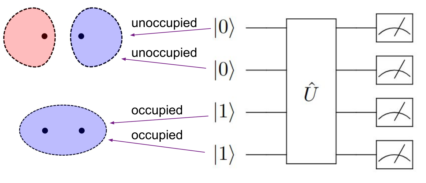
The mapping method creates a custom encoding of molecular electronic states onto quantum hardware that respects problem constraints (such as fixed electron number and spin multiplicity) while using fewer qubits than standard encodings like Jordan-Wigner.

Key Features

• Reduced Qubit Requirements: Constraint-based mapping significantly decreases the number of qubits needed to represent molecular systems
• Efficient Measurements: Novel measurement scheme reduces circuit complexity for Hamiltonian expectation value estimation
• No Approximations: Methods preserve the full physics of the quantum chemistry problem
• Classical Preprocessing: Resource-intensive calculations performed classically, executed only once per problem

Benefits

• Automatic Constraint Enforcement: VQE optimization is confined to physically valid states
• Faster Convergence: Smaller search space leads to more efficient optimization
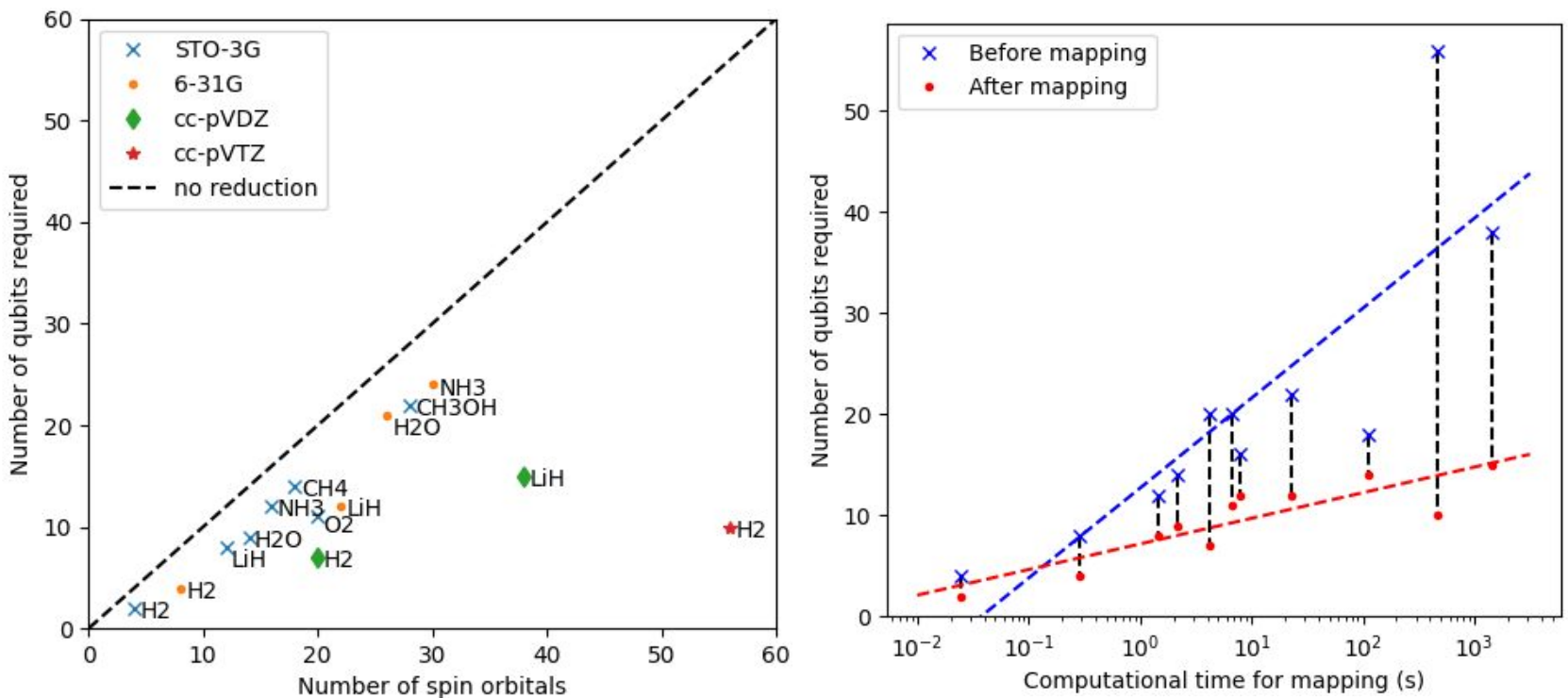
• Hardware Efficiency: Fewer qubits required, especially beneficial for larger basis sets
• Exact Results: No approximations to the underlying physics

How It Works

1. Define Constraints: Specify physical constraints for your molecular system:

2. Number of electrons (typically matching nuclear charge for neutral molecules)

3. Spin multiplicity (singlet, doublet, triplet, etc.)

4. Spatial symmetries (optional)

5. Identify Valid States: The method identifies the subspace of Fock space states that satisfy all constraints. For N spin orbitals and M valid states satisfying constraints, only \(log_2(M)\) qubits are needed instead of N qubits.

6. Generate Custom Mapping: A bijective mapping operator D is constructed that maps the valid subspace to computational basis states on the quantum computer.
7. Transform Hamiltonian: The molecular Hamiltonian is transformed to operate in the reduced Hilbert space: \(H_H= D H D^{\dagger}\)

TaskType: mol_map

• Inputs

geometry: array 1-d, list Geometry of molecule

symbols: array 1-d, list Element symbol (letters) for each atom in the geometry and in sequence how defined in the geometry. E.g. symbol for hydrogen is "H" for iron thek symbol is "Fe".

basis: string Basis set definition (Default: "sto3g")

multiplicity: value Spin multiplicity enforced by projection of the determinant wavefunction. E.g., to obtain a triplet state the value should 3, for the ground state the value should be set to 0.

charge: value Total charge of the molecule.

• Output

mapped_hamiltonian: array 2-d, list (float) The mapped Hamiltonian in sparse format. Each element has a list defining the row, column and value of each element in the Hamiltonian matrix.

hf_state: list (int) The Hartree Fock ground state in the new basis.

mapping_matrix: array 2-d, list (float) The mapping matrix \(D\) generated from the molecular Hamiltonian (Hilbert space). The matrix is a mapping from the Hilbert space to the subspace in sparse format. Each element has a list defines the row, column and value of each element in the mapping matrix \(D\).

Measurement method

Purpose

The measurement method efficiently evaluates the expectation value of the mapped Hamiltonian using a novel circuit generation scheme that groups terms by computational basis state pairs rather than Pauli string decomposition.

How it works

Express Hamiltonian in Basis States: The Hamiltonian is written as:

where \(\ket{m}\) and \(\ket{m'}\) are computational basis states.

Partition Terms: Terms are divided into two groups:

Diagonal terms (\(m = m'\)): Measured directly in computational basis Off-diagonal terms (\(m \neq m'\)): Require basis rotation circuits

Generate Measurement Circuits: For off-diagonal terms, circuits are grouped by which qubits differ between \(\ket{m}\) and \(\ket{m'}\):

Terms with the same "active qubits" are measured simultaneously Each group requires one Hadamard gate and CNOT gates Maximum of \(2M\) circuits needed (where \(M\) is dimension of mapped space)

Extract Expectation Values: Measurement probabilities combined with Hamiltonian coefficients yield \(\braket{H}\)

Benefits

• Fewer Unique Circuits: Typically requires fewer measurement circuits than Pauli string grouping methods
• Simultaneous Measurements: Multiple Hamiltonian terms measured per circuit
• Hardware Flexibility: Circuit topology can be adapted to quantum device connectivity
• Shallow Circuits: Measurement circuits have low depth, reducing decoherence effects

TaskType: qasm_gen

• Inputs

operator: array 2-d, list (float or int) The operator to be measured in sparse matrix format. The operator needs to be real valued and Hermitian. Each element should be a list defining the row, column and value of each element in the operator matrix.

• Optional Inputs

state_vector: array 1-d, list (float or in) A vector defining the state the operator should be measured in, such as the HF ground state. (Default behavior: no initial_state circuit generated) (default: None)

state_circuit: str/openQASM file The circuit defining the state for the expectation value measurement. (default: None)

include_state_circuit: bool Logical argument determining whether the generated qasm circuits should include the state preparation or not. If True, either state_circuit or state_vector needs to be defined. (default: False)

• Output

circuit_files: list (str) List of strings defining all circuits to be measured, in openQASM 2.0 format. If include_state_circuit was set to True, these circuits contain the combined state and measurement circuits. Ordered by circuit number.

postprocessing_instructions: array 2-d, list (float) The data needed to post-process the measurement results to arrive at the expectation value. The first index refers to the circuit number and the second to the qubit in the circuit.

To get the final expectation value with M=postprocessing_instructions:

• For each circuit in circuit_files, measure the occupation probability of each qubit.
• Create a matrix P, where P[i,j] is the probability of the i'th qubit of the j'th circuit.
• Matrix multiply M and P, and take the trace: (M@P).trace()

state_circuit: str Only available if state_vector input was defined. Circuit instructions for preparing the state defined in state_vector OpenQASM 2.0 format.

Combining the mapping and measurement methods

Combined Performance

When used together, the mapping and measurement methods provide synergistic benefits:

Molecule	Basis	Qubits (JW)	Qubits (Mapped)	Pauli Terms	Measurement Circuits
H2	STO-3G	4	2	14	2
LiH	STO-3G	12	8	630	25
H2O	STO-3G	14	9	1085	512
BeH2	STO-3G	14	11	665	1943
CH4	STO-3G	18	14	9260	16384

The number of measurement circuits after mapping approaches the theoretical maximum of \(2^Q\) where \(Q\) is the number of qubits after mapping, indicating the mapped Hamiltonians encode information efficiently.

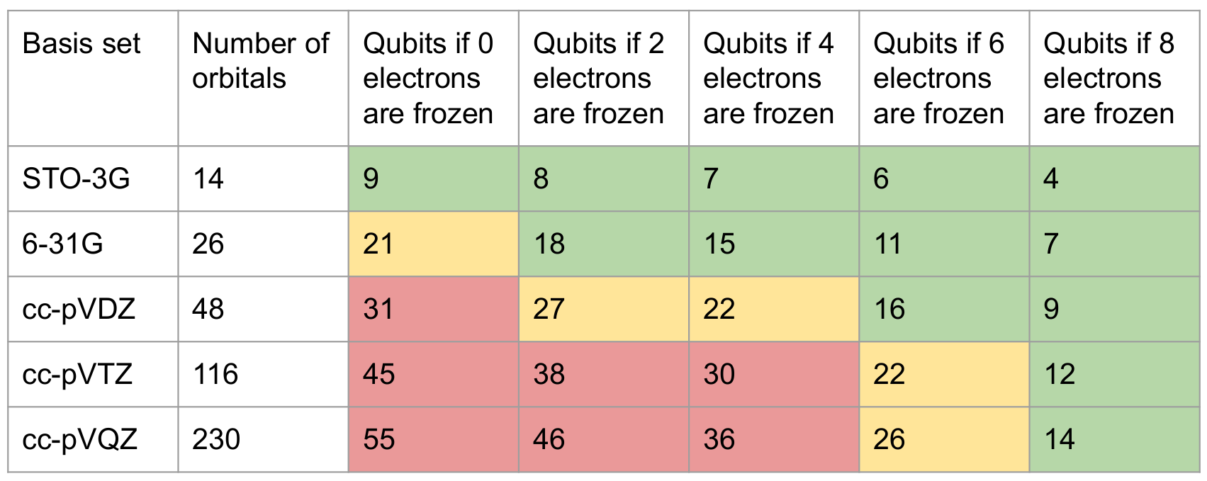
The following table shows the qubit requirements for water with respect to different basis sets and frozen orbitals:

Efficient quantum computing with parameterized tensor networks as matrix product states (MPS) and operators (MPO)

Tensor networks have shown that they can be applied to encode quantum chemistry problems in a highly efficient way to apply calculation routines for various molecular properties.

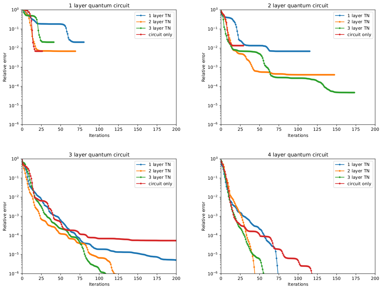
The TN-VQE method depicted in our paper ² was the starting point for us to develop a tensor network based approach to leverage classical computing to perform as much computational effort for a quantum chemistry calculation as possible to only make the most crucial calculation run on a QPU.

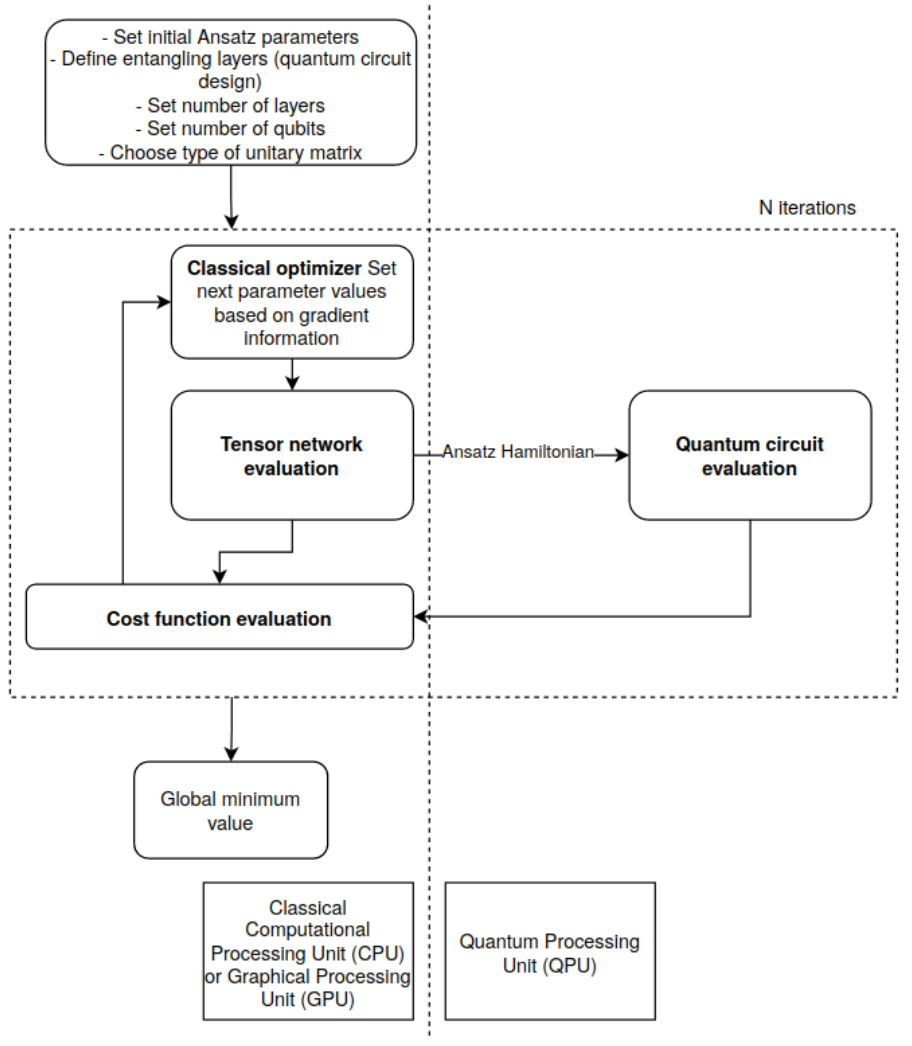
The Tensor Network-Assisted Variational Quantum Eigensolver (TN-VQE) is a hybrid quantum-classical algorithm that combines the strengths of tensor network methods with the Variational Quantum Eigensolver (VQE) to improve convergence and accuracy when finding ground state energies of quantum systems. The tensor network construction can be separated from the specific quantum algorithm (VQE) and one can combine the generated Hamiltonian in different ways with other algorithms.

Purpose

Traditional VQE algorithms face several challenges on current NISQ (Noisy Intermediate-Scale Quantum) devices:

• Barren plateaus: Optimization landscapes where gradients vanish, causing the algorithm to stall
• Initialization sensitivity: Poor choice of initial parameters can prevent convergence
• Shallow circuit limitations: NISQ devices require shallow circuits, limiting expressiveness

TN-VQE addresses these challenges by incorporating parameterized tensor networks to better represent the quantum many-body system before the quantum circuit optimization.

Benefits

• Improved convergence: TN-VQE demonstrates better convergence compared to randomly-initialized quantum circuits, particularly for circuits with fewer layers where standard VQE often fails to converge.
• Reduced circuit depth: The tensor network assists the quantum circuit by better encapsulating the complexity of quantum many-body systems, allowing accurate results with shallower circuit depths suitable for NISQ devices.
• Better gradient properties: The TN-VQE approach exhibits smaller gradient magnitudes during optimization, suggesting: More efficient parameter updates, a smoother optimization landscape and reduced sensitivity to noise in quantum simulations.

How It Works

The TN-VQE splits the optimization task between a classical tensor network and a quantum circuit. The minimization problem becomes:

\[E_{min} = min_{\theta,\phi} \braket{0|U^{\dagger}(\phi) U^{\dagger}(\theta) H U(\theta) U(\phi)|0}\]

where:

• \(U(\theta)\): Parameterized unitary tensor network (classical)
• \(U(\phi)\): Parameterized quantum circuit (quantum)
• \(H\): Problem Hamiltonian

• \(\theta, \phi\): Parameters optimized simultaneously

• Hamiltonian representation: The system Hamiltonian is encoded as a Matrix Product Operator (MPO).

• Unitary tensor network: A parameterized classical tensor network \(U(\theta)\) wraps around the Hamiltonian, improving its representation. Quantum circuit: A standard parameterized quantum circuit \(U(\phi)\) prepares quantum states.
• Joint optimization: Both \(\theta\) and \(\phi\) are optimized simultaneously using gradient descent.

TaskType: tn_qc_opt

• Inputs:

h_coeff_values: 1-d array (floats), list The coefficients of the Hamiltonian

h_operators: List The operators defining the Hamiltonian, the order should correspond to H_coeff_values. Can be in three forms:

• fermionic operators: List (tuples) Each Hamiltonian term (consisting of a string of fermionic creation and/or annihilation operators) is represented by a tuple of 2-tuples (each 2-tuple representing an operator). The first element of the 2-tuple is an integer, representing the site the operator acts on. The second element is a boolean: True (or 1) represents a creation operator, False (or 0) represent an annihilation operator See OpenFermion (https://quantumai.google/openfermion/tutorials/intro_to_openfermion) Example: a_4^\dagger a_2 a_1 = ((4,1),(2,0),(1,0)) or ((4,True),(2,False),(1,False))
• qubit operators: List (tuples) Each Hamiltonian term (consisting of a string of single qubit pauli operators) is represented by a tuple of 2-tuples (each 2-tuple representing an operator). The first element of the 2-tuple is an integer, representing the site/qubit the operator acts on. The second term is a string denoting the type of operator ('X', 'Y' or 'Z'). See OpenFermion Example: X_0 Y_1 Z_3 = ((0,'X'),(1,'Y'),(3,'Z'))
• qubit operators: List (strings) Each string represents a term, where each operator is denoted by the corresponding letter ('X', 'Y' or 'Z') followed by an integer represeting the site/qubit it acts on. The operators should be seperated by a space. Example: X_0 Y_1 Z_3 = "X0 Y1 Z3"

n_iterations: int Number of maximum iterations for optimization

n_layers_network: int Number of layers for the classical tensor network, parametarized by theta

• Optional Inputs:

qasm_ansatz: string QASM circuit ansatz as parameterized quantum circuit via directives with input arrays (Default: strongly entangled layers circuit)

n_layers_circuit: int Number of layers for the quantum circuit (parametarized by phi). (Default: 3 of qasm_ansatz is None, 1 otherwise)

three_para_tn: bool Logical arguments on wheter the rotation gates that make up the tensor network layers are parametarized by 3 parameters (arbitrary rotation) or 1 parameter (only phase rotation) (Default: True)

theta_init: array Initial guess for theta parameters (defining the tensor network ). (Default: zeros)

phi_init: array Initial guess for phi parameters (defining the quantum circuit ). (Default: random)

conv_tol: float Convergence tolerance

opt_method: string Currently the default is 'BFGS'. In the future other methods will be available.

backend: Definition of which device or simulator/emulator should run the quantum circuit. See possible options here: https://pennylane.ai/devices Examples (simulators): "lightning.qubit" (Pennylane simulator), "qiskit.aer" (Qiskit aer simulator) (Default: "default.qubit", Pennylane simulator)

• Outputs:

vqe_energy: float The ground state energy of the input Hamiltonian.

phi: array (floats) The values of the quantum circuit parameters phi reached during the optimization.

theta: array (floats) The values of the tensor network parameters theta reached during the optimization.

h_tn_opt_qubit: array (floats) The coefficients of the optimized tensor network Hamiltonian.

qubit_operators: array (strings) Each string represents a term in the optimized Hamiltonian in the following format: Each operator is represented by the corresponding letter ('X', 'Y' or 'Z') denoting its type, and an integer denoting which site/qubit it acts on. When a term involves more than a single operator, they are separated by a space.

When the MPS encoding has completed you can again, as shown with the mapping and measurement methods above, run a VQE routine. This also allows to combine the mapping, measurement and MPS encoding for the VQE routine.

To get a fermionic Hamiltonian from the outputs H_TN_opt_qubit and qubit_operators, one can use Openfermion:

from openfermion.ops import QubitOperator
from openfermion.transforms import reverse_jordan_wigner

# Initialize Hamiltonian
QB_ham = QubitOperator()

for pair in zip(qubit_operators,H_TN_opt_qubit):
    QB_ham += QubitOperator(*pair)

# Transform qubit Hamiltonian to a Fermionic Hamiltonian
FO_ham = reverse_jordan_wigner(QB_ham)
FO_ham.compress()

print(FO_ham)

#Extract the coefficients and operators for each term
fermionic_operators = FO_ham.terms.keys()
H_TN_opt_fermionic = [FO_ham.terms[label] for label in fermionic_operators]

Correlation optimized virtual orbitals (COVO)

The COVO method addresses a fundamental challenge in quantum computing simulations of molecular systems: reducing the dimensionality of the problem while capturing significant electron correlation. Traditional approaches using Hartree-Fock virtual orbitals often fail to capture meaningful correlation energy, particularly when using plane-wave basis sets where virtual orbitals tend to be scattering states with weak interactions.

COVO generates optimized virtual orbital spaces specifically designed to capture electron-electron correlation efficiently, enabling accurate quantum chemistry calculations with far fewer orbitals than conventional methods.

Key Features

• Efficient Correlation Capture: Captures significant correlation energy with a minimal number of virtual orbitals (typically 4-18 orbitals)
• Plane-Wave Compatibility: Specifically designed to work with pseudopotential plane-wave Hamiltonians, extending quantum chemistry methods beyond traditional atomic basis sets
• Systematic Convergence: Demonstrates steady convergence toward benchmark results as more virtual orbitals are added
• Quantum Computing Ready: Dramatically reduces qubit requirements for near-term quantum devices while maintaining accuracy
• Pairwise Optimization: Generates virtual orbitals by optimizing small configuration interaction (CI) Hamiltonians containing pairwise electron correlations
• Periodic System Extension: Can be extended to periodic systems using Filon integration strategies for exact exchange and Brillouin zone integration

Benefits

Reduced Computational Cost: With just 4 COVOs, the method can recover a significant portion of correlation energy comparable to much larger basis set calculations (e.g., matching cc-pVTZ results with only 4 virtual orbitals for H2).

Near-Term Quantum Device Compatibility: By reducing the number of required qubits while maintaining accuracy, COVO makes quantum simulations feasible on current noisy intermediate-scale quantum (NISQ) devices.

Versatile Applications: The optimized orbital spaces can be used with various many-body methods including: - Full Configuration Interaction (FCI) - Coupled Cluster (CC) theory - Møller-Plesset perturbation theory - Variational Quantum Eigensolver (VQE) - ADAPT-VQE

Extensivity: Maintains proper size-extensivity for dissociated systems, with errors decreasing systematically as more COVOs are included.

How It Works

The COVO algorithm generates virtual orbitals sequentially by optimizing small select CI Hamiltonians:

1. Initialization: Start with filled Hartree-Fock orbitals from a reference calculation

2. Pairwise CI Construction: For each virtual orbital to be optimized (φᵥ), construct a small CI Hamiltonian containing:

3. The ground state filled orbitals
4. The current virtual orbital being optimized

5. Configuration state functions representing electron pairs

6. CI Diagonalization: Diagonalize the CI matrix to obtain expansion coefficients and the lowest eigenvalue

7. Gradient Optimization: Calculate the gradient of the energy with respect to the virtual orbital and update using conjugate-gradient or similar optimization methods

8. Orthogonality Constraint: Ensure the new virtual orbital remains normalized and orthogonal to all previously computed filled and virtual orbitals

9. Iteration: Repeat for the next virtual orbital until the desired number of COVOs is generated

TaskType: covo

• Inputs:

geometry: 1-d array, list Cartesian coordinates (x,y,z), in angstroms, representing the 3D position of all atoms (e.g., [0.0000, 0.0000, 0.0000, 0.0000, 0.0000, 0.6000])

symbols: 1-d array, list Atomic elements (e.g., ["H","H"]) that directly correspond to the coordinates in the geometry array.

cell_size: value (float) The dimension of the simulation box, in Ångstroms [Å].

periodic: True/False Boolean flag indicating whether the system is an infinite repeating lattice (True) or an isolated molecule (False)

cutoff: value (float) Energy cutoff threshold used to truncate the basis set.

n_virtual_orbitals: value (integer) The number of unoccupied (virtual) molecular orbitals to include for advanced correlation or active space calculations.These are the COVO orbitals to be optimized.

charge: value (integer) The net electric charge of the system (e.g., 0 for neutral, -1 for an anion).

multiplicity: value (integer) The spin multiplicity of the system, defined as M = 2S + 1 (e.g., M=1 for a singlet state with all electrons paired with S=0).

tolerance: value (float) The numerical convergence threshold for the Self-Consistent Field (SCF) iterations.

• Outputs:

one_electron_integrals: array 2-d (float) A matrix (N x N) containing the kinetic energy and nuclear attraction terms for individual electrons within the basis set.

two_electron_integrals: array 4-d (float) A tensor (N x N x N x N)representing the electron-electron repulsion interactions.

hf_energy: value (float) The molecular ground-state energy [Hartree] calculated using the mean-field Hartree-Fock approximation.

fci_energy: value (float) The exact ground-state energy (Hartree) within the chosen COVO optimized virtual orbitals, calculated via Full Configuration Interaction.

vqe_energy value (float) The optimized energy (Hartree) computed using the Variational Quantum Eigensolver (VQE) algorithm with the chosen COVO optimized virtual orbitals.

hamiltonian: array 2-d (float) The matrix representation of the system's electronic Hamiltonian, mapping the total energy operators.

Zero-noise Extrapolation for Variational Quantum Algorithms

Variational Quantum Algorithms (VQAs) like the Variational Quantum Eigensolver (VQE) are specifically designed to run effectively on near-term quantum computers, which lack quantum error correction. Consequently, there’s substantial interest in determining whether these algorithms can provide practical computational advantages. In chemistry, accurately predicting molecular energies with classical methods (such as Density Functional Theory, Coupled Cluster, and Full Configuration Interaction) can be extremely computationally expensive. Quantum computing, with its natural ability to represent quantum entanglement and correlations between particles, has the potential to significantly accelerate these calculations. Thus, enhancing VQAs through error mitigation methods such as Zero-noise Extrapolation (ZNE) is relevant to areas such as pharmaceuticals, energy, and catalysis – which together have a global market size of trillions of dollars – for molecular and material design both in industry and academic research.

ZNE works by intentionally increasing noise in quantum circuits via redundant gates, measuring the expectation value of a circuit with respect to some operator at different noise levels, and then extrapolating with a curve fit to estimate the zero-noise result.

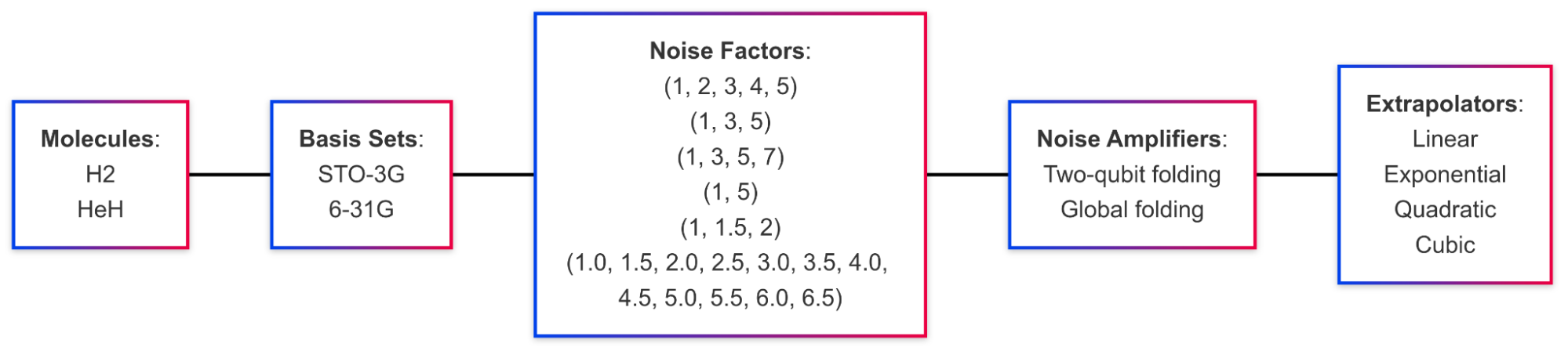
MQS has systematically benchmarked different ZNE configurations – combinations of noise factors, noise amplification methods, and extrapolation techniques – to identify which configurations yield the most accurate and reliable improvements to VQE, as well as which configurations lead to unrealistic energy estimates.

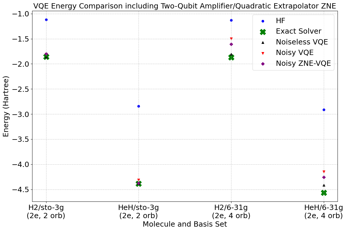
We ran a series of experiments to benchmark various ZNE configurations for VQE using Qiskit and classical simulation with the IBM Brisbane noise model. From the experiments run, the best-performing ZNE configurations for the analyzed VQE cases in terms of stability and accuracy involve a large number of noise scalars (such as 12 factors between 1 and 6.5), two-qubit gate folding, and quadratic extrapolation. The cubic and exponential extrapolation methods can be prone to producing unphysical energies. By mapping which options consistently converge toward the noiseless energy and which diverge, a recipe for reliable error mitigation in VQE is provided.

ZNE can help one progress towards chemical accuracy with VQAs as shown in our results from the best-performing configuration. Note that this experiment was not tuned for chemical accuracy, it simply demonstrates how ZNE can take one closer to that target.

Genetic gate-based quantum circuit generation

See Xenakis repository: Link

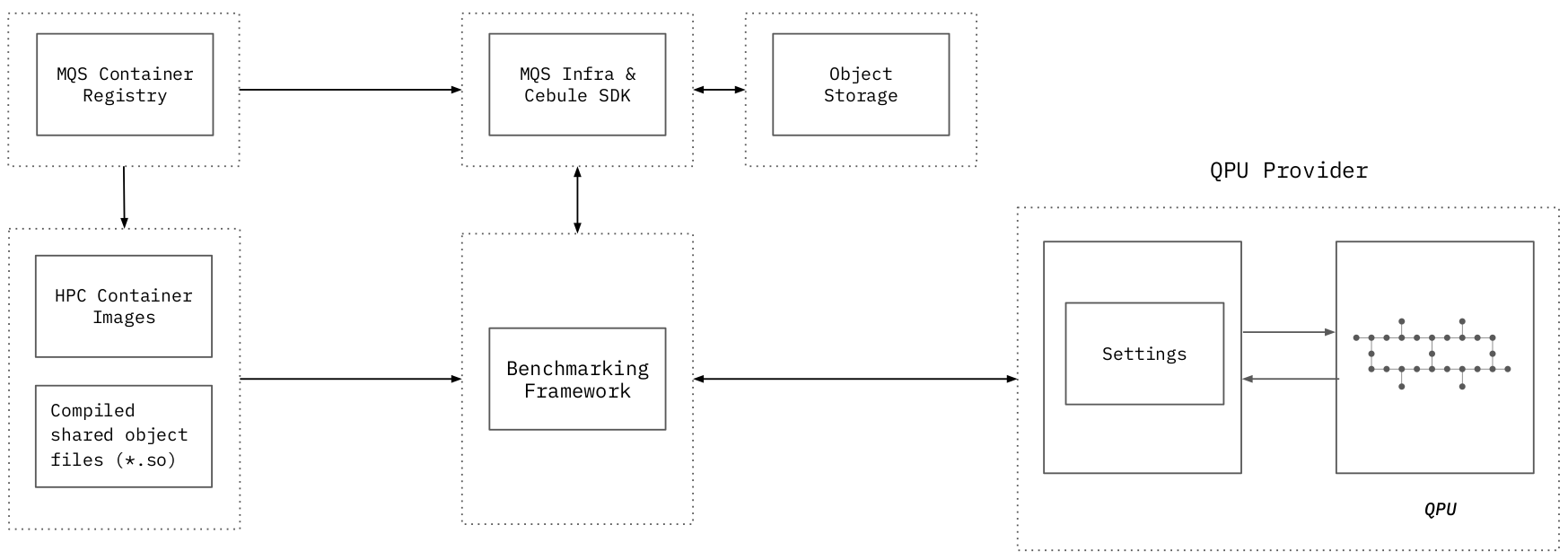
Benchmarking framework

Quantum computing research articles from MQS

• Resource efficient method for representation and measurement of constrained electronic structure states with a quantum computer
• A joint optimization approach of parameterized quantum circuits with a tensor network
• Comparative Studies of Quantum Annealing, Digital Annealing, and Classical Solvers for Reaction Network Pathway Analysis and mRNA Codon Selection
• Quantum phase estimation with optimal confidence interval using three control qubits

Completed and current MQS projects:

PhotoQ: Photonic quantum computing project involving measurement-based quantum computing and Gaussian boson sampling (GBS).

DLR Quantum Computing Initiative - QuantiCoM Project: Advanced water simulations with classical and quantum computing.

Q-Chemion: end to end quantum computing calculation pipeline with QEDMA, Oxford Ionics, Copenhagen University and the Technical University of Denmark (DTU).

MQS x Fraunhofer SCAI Benchmarking Framework: In collaboration with Fraunhofer MQS has developed a quantum computing algorithms benchmarking framework to assess methods related to quantum computing enhanced quantum chemistry calculations (to be released).

Quantum Innovation Challenge: Quantum Innovation Challenge in collaboration with Novo Foundation, BioInnovation Institute (BII), DCAI, QAI Ventures and many more. The annual challenge focuses on applications of quantum computing within the life sciences.

Q-ARMOR - Quantum-AI Assisted Rational Design of Metallopeptide Conjugates Against Antimicrobial Resistance

---

1. Kaur Kristjuhan and Mark Nicholas Jones. Resource efficient method for representation and measurement of constrained electronic structure states with a quantum computer. 2023. URL: https://arxiv.org/abs/2303.01122, arXiv:2303.01122. ↩

2. Clara Ferreira Cores, Kaur Kristjuhan, and Mark Nicholas Jones. A joint optimization approach of parameterized quantum circuits with a tensor network. 2024. URL: https://arxiv.org/abs/2402.12105, arXiv:2402.12105. ↩↩